Batch Evolution Modeling:

Overview

In this post, I go over applications of batch evolution modeling, used in process monitoring. What is batch evolution modeling? Batch evolution modeling is a framework of methods that allow us to track processes holistically, evaluate batches in progress, and predict final outcomes. It incorporates concepts from data science/machine learning as well as (multivariate) statistical process control. Although the context is in biomanufacturing and bioprocess engineering, the concepts can be applied to other fields for process monitoring and anomaly detection (manufacturing, forecasting).

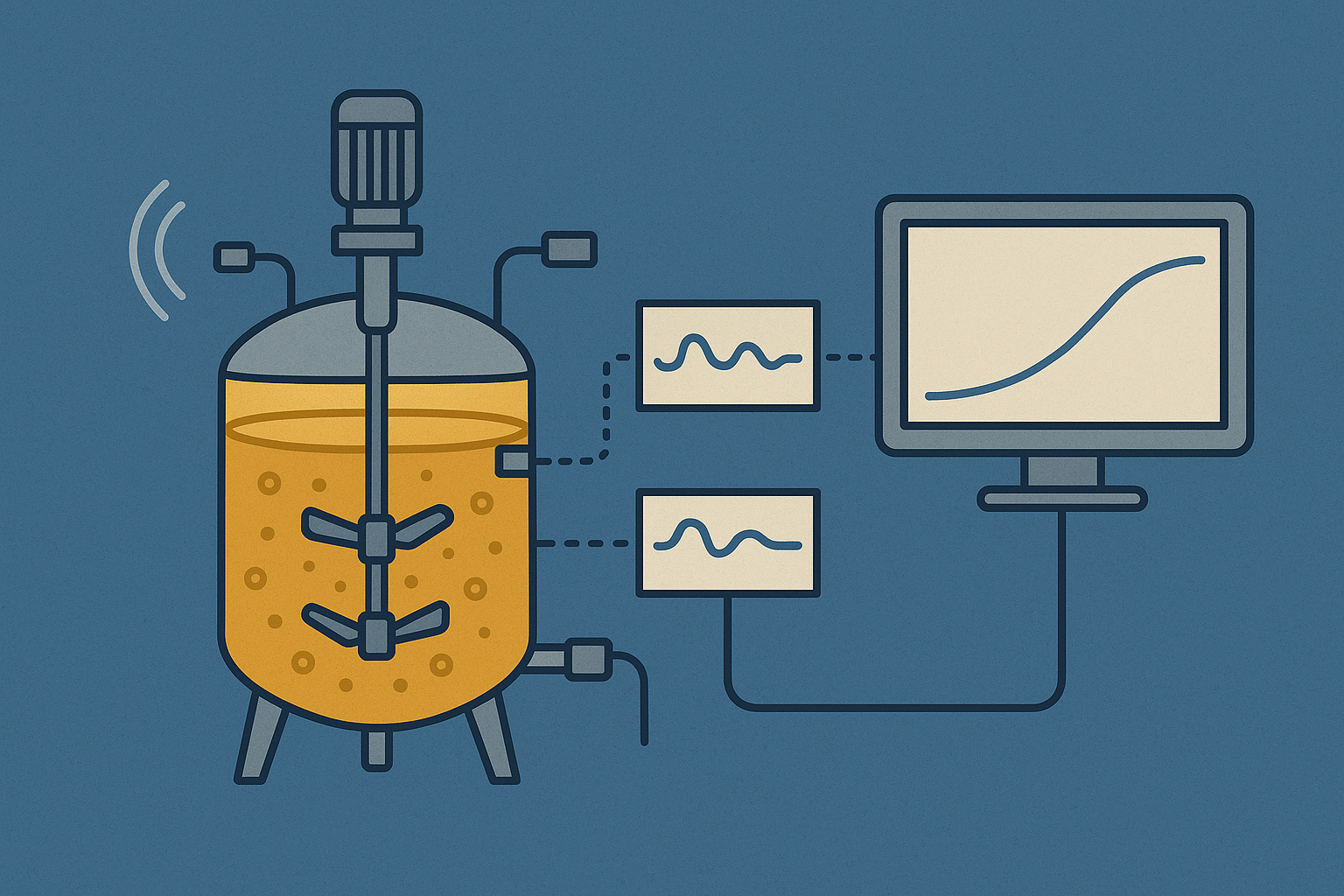
jmp_auc — Batch in-progress being monitored.

What are some use cases? Let’s say we have an established process that we are running periodically. As we generate data from runs, we establish a “Golden Batch” trajectory - or how a run is supposed to trend. What’s ‘normal’ for a ‘good’ batch? How do we tell if a batch in-progress is behaving ‘normally’ or deviating? Crucially, if it is deviating, can we diagnose it early enough to intervene, or do we have enough evidence to ‘scrap’ the batch immediately, saving time and costs? We can answer all of these with batch evolution modeling! Existing software (SIMCA) lets you do this - here I implement this in Python.

Data and code as well as reference literatures can be found on my Github.

Introduction

In this scenario we work with a synthetic dataset of 17 runs based off a real world bioprocess where we are making antibody as a product in a bioreactor. Along the way, samples are taken and measured for product concentration (titer in mg/mL units) as well as metabolites. It is common to collect sensor data such as dO%, pH, agitation speed, temperature, etc. In this example, we monitor 5 metabolites (acetate, glucose, ammonia, phosphate, pyruvate). We can familiarize ourselves with the trends with exploratory data analysis.

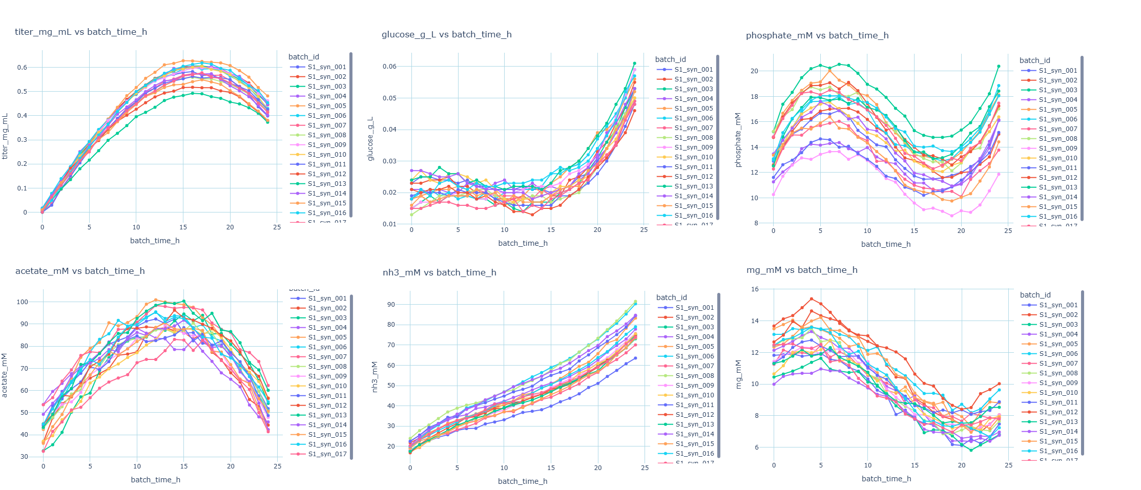
titer and metabolite trends — Titer and Metabolite Trends

We can tell the process is a reaction with hourly sample points over the course of 24 hours. Titer rises and maxes out at around 16 hours, then falls, likely due to dilution effects. Other metabolites have different profiles. Keep in mind this is a cleaned and simplified synthetic data set.

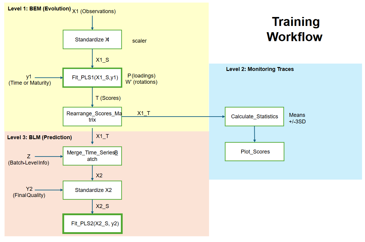
Step 1 - Batch Evolution Modeling - Training

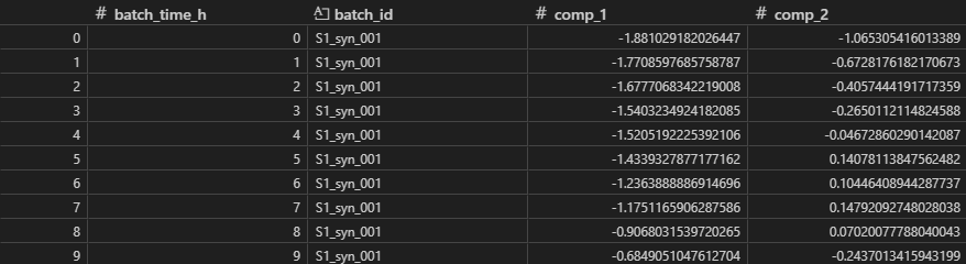
After compiling all historical ‘good’ batches into our dataframe below, we must preprocess the data further before training our model.

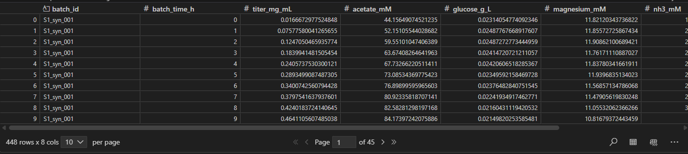
First, we ensure the data is in the right format, where each batch and sample point make up rows while features, or measurements make up columns. We’ll denote this as N batches, J sample points, and K measurement columns. The resulting matrix has N x J rows and K columns. We define Y as process maturity - in this instance we use batch_time.

Data Preprocessing

    import numpy as np
    import pandas as pd
    import matplotlib.pyplot as plt
    from sklearn.preprocessing import StandardScaler
    from sklearn.cross_decomposition import PLSRegression
    import sklearn.model_selection as skm
    import plotly.graph_objects as go

    df = pd.read_excel("synthesized_data.xlsx")
    X_cols = ['acetate_mM', 'glucose_g_L', 'magnesium_mM', 'nh3_mM', 'phosphate_mM']
    batch_col='batch_id',
    time_col='batch_time_h',
    y_time_col='batch_time_h',
    df_model = df_train[[self.time_col, self.batch_col] + self.X_cols].copy()
    df_model = df_model.sort_values([self.batch_col, self.time_col])
    X = df_model[self.X_cols].to_numpy()
    y = df_model[[self.y_time_col]].to_numpy()  # time as y

Next, we standardize X. This is important because different features have different magnitudes and we want to avoid features with high values from dominating. Geometrically, centering at 0 allows us to interpret as distance from origin (which is nice for calculations). We can use sklearn library here.

    self.scaler_X = StandardScaler()
    X_scaled = self.scaler_X.fit_transform(X)

Next we initialize the Partial Least Squares (PLS) Model.

What is PLS?

Partial Least Squares (PLS) is a supervised regression method used when you have many, often correlated predictors (X) and want to predict one or more responses (Y). It’s commonly used in chemometrics, spectral analysis, and omics/gene work because it handles high dimensional data and collinearity well. Like PCA, PLS builds latent components (scores and loadings) that are linear combinations of the original X-variables. However, instead of just capturing the variance in X, PLS chooses these components to maximize the covariance between X and Y, meaning it finds the variation in X that is most useful for predicting Y. The model is composed of the following components:

$X = TP’ + E$

$y = Tc + f$

X are the inputs.
y is the output.
T is score matrix. These are the new ‘features’ describing the state of the batch. It’s calculated by X.dot(W) (where W is the projection matrix that maps from X space to A space)
P,c are the loadings for X and y.
E, f contain the residuals.

In batch evolution, local time is used as the Y-variable: it forces the PLS model to find the specific variation in the process variables (X) that describes the evolution of the batch over time.

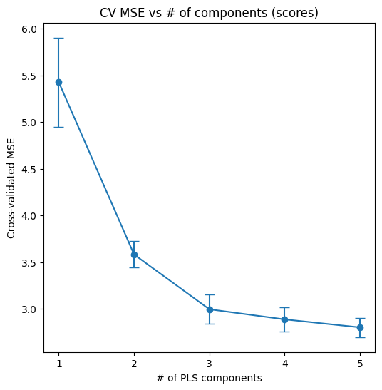
Choosing number of components

To determine the number of components to use, we use cross validation and fit models with 1,2,3… components, and plot prediction error vs number of components. We choose the point where error stops improving meaningful (the “elbow”), balancing good prediction performance against overfitting.

    kfold = skm.KFold(n_splits, random_state=0, shuffle=True)
    pls = PLSRegression()
    param_grid = {'n_components': range(1, max_components + 1)}

    grid = skm.GridSearchCV(
        pls,
        param_grid,
        cv=kfold,
        scoring='neg_mean_squared_error'
    )
    grid.fit(X_scaled, y)

Finalize model and get scores

2 components is sufficient here. After choosing number of components, we can specify 2 components and finalize the model.

    self.pls_scores = PLSRegression(n_components=self.n_components)
    self.pls_scores.fit(self._X_scaled_scores, self._y_scores)
    X_scaled=self._X_scaled_scores
    T = self.pls_scores.transform(X_scaled)  #these are scores.
    P = self.pls_scores.x_loadings_ #loadings

The scores are captured in T, with dimensions (NxJ)xA.

So we have constructed a PLS model (pls_model_1) that fits to a training set of ‘good’ batches. We’ve extracted a scores matrix, which is a compressed form of the data that best summarizes variation in X that drives the process forward in time.

Step 2 - Batch Traces and Monitoring

Rearrange data and calculate summary metrics

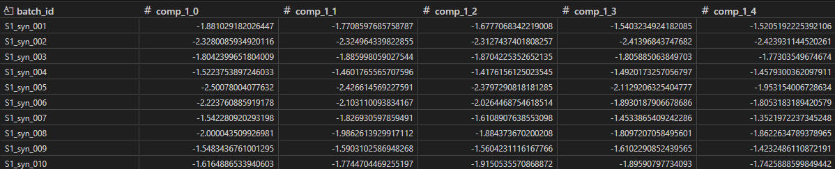
Next, we rearrange the scores matrix to wide form, X_T, with dimensions Nx(AxJ).

long = pls_scores_df.melt(
    id_vars=[batch_col, time_col],
    value_vars=comp_cols,
    var_name='component',
    value_name='score'
)

wide = (
    long
    .pivot(index=batch_col, columns=['component', time_col], values='score')
    .sort_index(axis=1, level=[0, 1])
)

There should be 1 row for each batch, and 1 column for each component x time point.

Using X_T, we can calculate metrics such as average and standard deviations to use in our control charts. We do this for each component and time point. With this format, it is easy to establish averages and upper/lower bounds for ‘good’ batches as they evolve over time. For the bounds, we use +/-3 SD.

Monitoring incoming batches

Now we can plot incoming batches against the training set and upper/lower bounds and determine whether they are behaving or deviating.

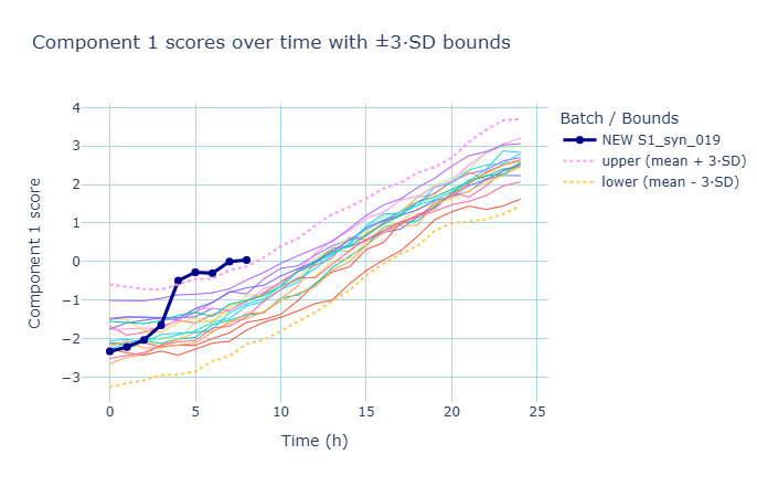
For example, if an incoming batch deviates by crossing the threshold of +3SD in component 1, it’s very likely not a ‘good’ batch. By using batch evolution modeling, an engineering supervisor can make the decision to scrap the batch mid-run, saving substantial time and masterial costs

Contribution Scores

Once we detect a deviation (the trace crosses the +3SD limit in component 1) - we can examine what caused it?. We answer this by calculating contribution scores. Conceptually we can think of contribution as the weight of the variable (W) multiplied by how far the variable is deviating from the average (X_scaled).

    x_raw = row[self.X_cols].to_numpy().reshape(1, -1)
    x_scaled = self.scaler_X.transform(x_raw)  #(1xk)
    w = self.pls_scores.x_rotations_      #rotations
    w_a = w[:, comp_index].reshape(1,-1) #(1xk)
    contrib_scaled = x_scaled * w_a         # (1xk)

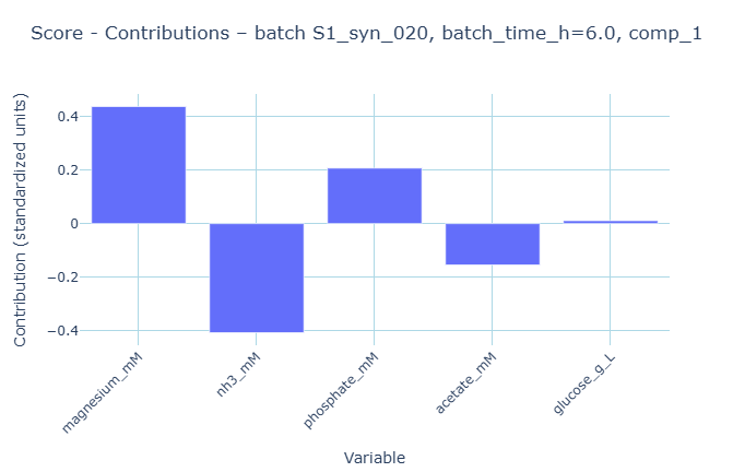
These contributions show which value is driving the score to be high at that point. The plot indicates acetate has a positive contribution to the component 1 score. We can confirm this by examining the data and find indeed, there was an acetate spike for that time point. So effectively after a deviation is detected (crossing the threshold), we can diagnose what contributed to this deviation. Keep in mind, contributions can show up in different components - it all depends in how the model decomposed the data. In batch evolution modeling, it’s common for component 1 to represent batch maturity, and for componenet 2 to represent quadratic evolution (shape).

So we have established a normal range for ‘good batches’, and used summary statistics in component space to detect deviations. We then use the contributions to diagnose what contributed to that deviation. Crucially, we can quickly utilize this approach during an ongoing batch to determine whether a batch is ‘deviating’ based on a set threshold.

Step 3 - Batch Level Modeling

We’ve used batch evolution to summarize and monitor batches across a time series. Now we extend the analysis to batch level modeling, where we use our time series data as well as our background data (such as initial conditions) to predict an outcome (such as final titer). We take the scores (X_T), merge (place side-by-side horizontally) with our background data (Z), to get X2, which also has one row for each batch.

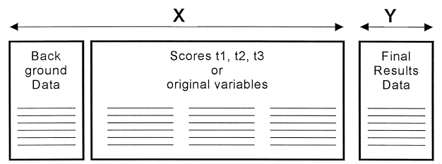
With this we train another PLS model (PLS2). Now we can use PLS model 2 to predict titers for a test set. For prediction of new batches, we first pass new raw time-series data through our Step 1 model to extract the scores (X_T). These scores are what we merge with Z to feed into the Batch Level Model.

An important application of this can be to get an early readout, and examine if a batch likely has low yield, while waiting for the official result to come in.

Continuous monitoring

Finally, a model is only as good as the data it was trained on. It’s important to contiously monitor the model for drift (aging equipment, introduction of new raw materials, etc). The training set should be updated periodically to reflect the current process reality.

Visual Representation (Flow Diagram)

Follow-up Questions

What happens if the sampling points dont line up?

This is often the case in the real world, where sampling doesnt happen exactly on the hourly interval. These methods are robust and can handle uneven sample points. Because PLS1 predicts batch maturity, we can train the model on unaligned data. The model then can predict y_pred (batch maturity) for all sample points. Then we can align data points on batch maturity axis at regular intervals (0,10,20,30%..) using interpolation. Once aligned, we can then calculate the control limits.

Can we make early predictions on final outcomes on ongoing batches?

Yes! Essentially we can train on sub-models up to intermediate points (e.g. “10-hour model”.)

Why is +/-3 SD chosen as intervals?

+/-3 SD bounds are used in batch evolution modeling because they define strict boundaries of the “normal pattern of evolution” with a high degree of certainty (taking elements from statistical process control). Batches that cross these boundaries are “definite deviators”. We could also use +/-2 SD for more stricter controls.

Are there statistical indicators for batch similarity?

DmodX (Distance from Model X), Hotelling’s T2 are often used and represent deviation from ‘good batches.’

When is batch evolution modeling NOT useful?

When you lack a definition of “Normal”. Batch evolution modeling relies on historical reference data that you can confidently label as “good”.
If you’re only monitoring few variables. If you’re only monitoring 2 or 3 variables, you might as well plot the original variables. BEM shines when you need to summarize the interaction of many variables into a single trajectory.
When Alignment is Impossible. BEM assumes there is some evolutionary trajectory that can be aligned to a maturity axis.
When the process is “Steady State”. BEM is designed for processes that have a start and an end.

Ending Thoughts (What did we accomplish)?

In this guide, we leveraged batch evolution modeling to holistically evaluated processes.

Scores & Components - We used Partial Least Squares (PLS) to compress high-dimensional, noisy data into “Scores” that represent the state of the process.
Golden Batches - We constructed a model based off a training set of historical good batches, creating a trajectory that defines “normal.”
Health Monitoring - We can instantly apply the trained model to evaluate ongoing batches to assess their health.
Predicting outcomes - We extended to batch level monitoring (PLS2) to be able to predict final outcomes of a batch.
Open Source Stack - We achieved this using Python, sklearn, numpy, pandas.

Why this is important? Industrial data is often complex and heavily correlated. By using batch evolution modeling, we can evalute the process holistically. Some advantages include:

Early Detection -: We can see a batch drifting out of the “Golden Tunnel” hours before a single sensor hits an alarm limit
Interpretability -: When a deviation occurs, we don’t just guess; we can look at the Variable Contributions to see exactly which combination of signals caused the problem.

References:

S. Wold et al. Chemometrics and Intelligent Laboratory Systems 44 (1998) 331–340

https://www.sartorius.com/en/knowledge/science-snippets/understanding-the-basics-of-batch-process-data-analytics-507206

https://scikit-learn.org/stable/modules/generated/sklearn.cross_decomposition.PLSRegression.html